Loss Functions
When building a new deep learning model, there are four fundamental things that must be chosen:
- Data: What will the model be trained on?
- Architecture: What is the underlying structure of the model?
- Loss Function: How can we evaluate how well the model is doing?
- Optimizer: How should we make changes to the model to make it better?
What is a loss function?
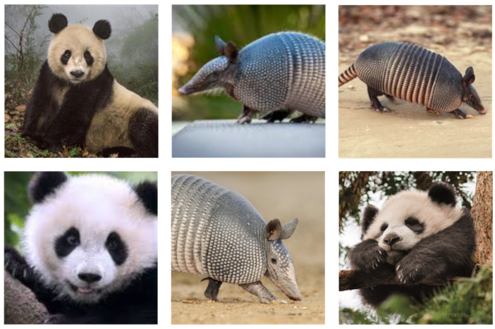
Let’s think about a simple classifier. We have a big pile of pictures that are either a picture of a panda or an armadillo and we want our network to be able to sort them into two piles:
Let’s say we show the neural network 100 of these pictures and it makes predictions about the content of each one. We want a way of knowing how good these predictions are.
Idea 1: Counting
The easiest way of assesing performance it to simple count how many correct predictions the network made. For example: “Of the 100 pictures, our network correctly classified 62 of them.”
We add a bit of detail by also counting the following:
- What percentage of pictures classified as pandas were actually pandas? (True positives)
- What percentage of pictures classified as pandas were actually armadillos? (False positives)
- What percentage of pictures classified as armadillos were actually armadillos? (True negatives)
- What percentage of pictures classified as armadillos were actually pandas? (False negatives)
This allows us to use a method of scoring called precision & recall. The precision is the ratio of true positives to total predictions and the recall is the ratio of true positives to total positives. The harmonic mean of the precision and recall is called the F score. A higher F score means a more accurate model.
The precision and recall technique has one big problem in the context of deep learning. It is non-differentiable. This means that, although precision and recall can tell us how good the predictions are at the moment, they can’t be used produce a gradient which can train the model.
Idea 2: Change To Classifier Confidence
We can do slightly better by having the network output how confident it is for its predictions for each individual image. For example, the network might say the following:
“I am 88% sure that image 6 is a panda”
or
“I am 3% sure that image 2 is a panda”
and in terms of training, we may respond:
“Well done! Image 6 was a panda, but update your parameters so next time you are closer to 100% sure, rather than 88%.”
or in the case of the second example:
“Well done! Image 2 was an armadillo. Next time try and aim for a 0% confidence instead of 3%”
(If the second example doesn’t make sense remember that an output of “0% panda” is equivalent to “100% armadillo”.)
This is the first example we have come across of a loss function. A loss function lets us combine two numbers (the model’s prediction and the actual label) into one number. The simple loss function above finds the difference between the prediction and the label (100% - 88% = 12% for example 1 and 3% - 0% = 3% for example 2. In practice these are outputted as decimals 0.12 and 0.03.)
The errors calculated by the loss function are known as the loss. We want to minimise the error and so a loss closer to 0 is better.
Unlike precision & recall, loss functions are differentiable and so our model can be trained! (As precision & recall is non-differentiable, it is called a metric and not a loss function).
By combining all of this, we can now understand why loss functions are so useful. They are differentiable functions that produce one number describing how accurate our current model is.
Loss functions in action
Mean Absolute Error
The loss function in the example above considers the raw difference between the model prediction and true label (100% - 88% = 12% for example 1 and 3% - 0% = 3% for example 2.) This is called absolute error. We often want to combine the accuracies of many of our model’s predictions at once. One way of doing so is taking the mean. For our example, this would be $ (12\% + 3\%) \div 2 = 7.5\%$.
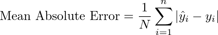
Unsuprisingly, taking the mean of a series of absolute errors is known as mean absolute error and is written mathematically like this:
Clearing this up with some annotation:
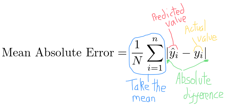
(The eagle-eyed with some calculus understanding may spot that mean absolute error is not differentiable when the error is 0. This isn’t really an issue as the loss will almost never be exactly 0.)
One issue with mean absolute error is that all errors are treated ‘equally’. Often we will want to penalise larger errors significantly more than small ones. The mean squared error loss function lets us do so.
Mean Squared Error
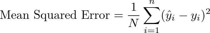
By changing the absolute difference in mean absolute error to a squared difference, we can easily write down the loss function for mean squared error.
Again, adding in some annotation:
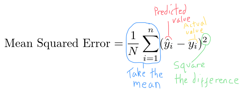
The squared term means that larger differences between $\hat{y}_i$ and $y_i$ will contribute far more to the final value of the loss function than smaller differences.
Classification & Cross-Entropy
The mean squared and mean absolute error loss function are most suited to a type of prediction known as regression.
When ever we are using our network to predict a continuous value (like the price of a house or a person’s height) we are performing regression. This is opposed to classification where we try to predict the class of something (e.g. What breed of dog is in this picture? Is this picture a panda or an armadillo?).
As discussed in the above section about probabilities, the output of a classfier will be a number between 0 and 1. When performing classification, the most common loss function used is cross-entropy. For the binary classification panda-armadillo problem, it looks like this:
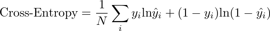
In the context of our example where $y_i=1$ is a picture of a panda and $y_i =0$ is a picture of an armadillo, we can add the following annotations:
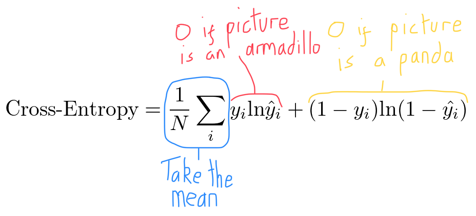
Again, the loss functions gives us one number that represents how accurate our network is.
Further Extenstions
The above is very small peak into the loss function zoo. There are many simple extensions of the loss functions presented above, such as mean absolute percentage error, hinge loss and logistic loss. Things can also get far more complex.
For example, in a Generative Adversarial Network (GAN) two neural-networks are actively fighting against each other. The loss function for the first neural network produces a better value not only when the first network performs better, but also when the second network performs worse (and vice versa). To obtain one coherent loss function for the whole system, the two individual loss functions must be combined into a mini-max problem.
It is likely that as machine learning architectures become more complex, the loss functions used will do the same. However, as the above has shown, the core question that all current loss functions address is the same: what function can we use to obtain one differentiable number that represents how accurate our network is?