Training GANs Using Wasserstein Distance
Generative Modelling
Over the years, us humans have become quite good at quickly analysing data. With any luck, you and I should easily be able to tell apart a picture of a cat from a picture of a dog. This is something so easy that it takes us only milliseconds to do and even young children can do so. Untill recently, getting computers to do the same has been near impossible. It is only in the last decade that any tangible progress has been been made. Nonetheless, for simple image recognition tasks, computers have now reached a stage where they are at a human-ish level.
Now let’s think about a different problem. I want you to draw for me a dog. Not a rough cartoon of a dog, but an actual photorealistic drawing. Not so easy, right? Looking at how long it took to get computers to be able to recognise cats from dogs, it’s easy to think that getting a computer to create an image of a dog that is as realistic as the one in the image below would be many decades away. You would be wrong.
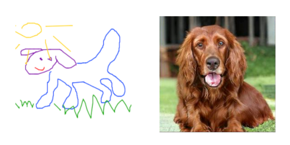
The dog on the right has never existed in any shape or form. It was generated in this paper.
The field of trying to get computers to generate data that is indistinguishable from real data (whether that be pictures, audio, text etc.) is known as generative modelling.
GANs & KL Divergence
A breakthrough in generative modelling came with the introduction of the Generative Adversarial Network, or GAN for short. A GAN is a specific architecture of neural network that learns to produce fake data by mimic the underlying probability distribution of some real data.
As the GAN aims to copy a real probability distribution, we need a loss function that can tell us how different two probability distributions are (the true PDF and the generated PDF). Compairing the similarity of two PDFs isn’t straightforward. The simplest way is to use a metric called the Kullback-Leibler divergence.
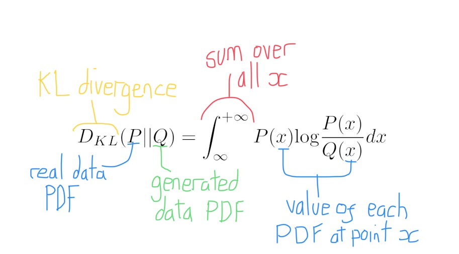
Although simple to calculate, the KL divergence is flawed. Note that the KL divergence between $P(x)$ and $Q(x)$ is different from the KL divergence between $Q(x)$ and $P(x)$. This is like saying the distance from London to Manchester is different from the distance from Manchester to London.
Note: To all intents and purposes, when we say the distance between two probability distribution, we mean the dissimilarity between them.
The fault is known as the asymmetry of KL divergence. There are other issues with KL divergence. Most notably, when our generated probability distribution is undefined at a point (i.e $Q(x) = 0$) then the KL divergence shoots off to infinity.
Jensen-Shannon Divergence
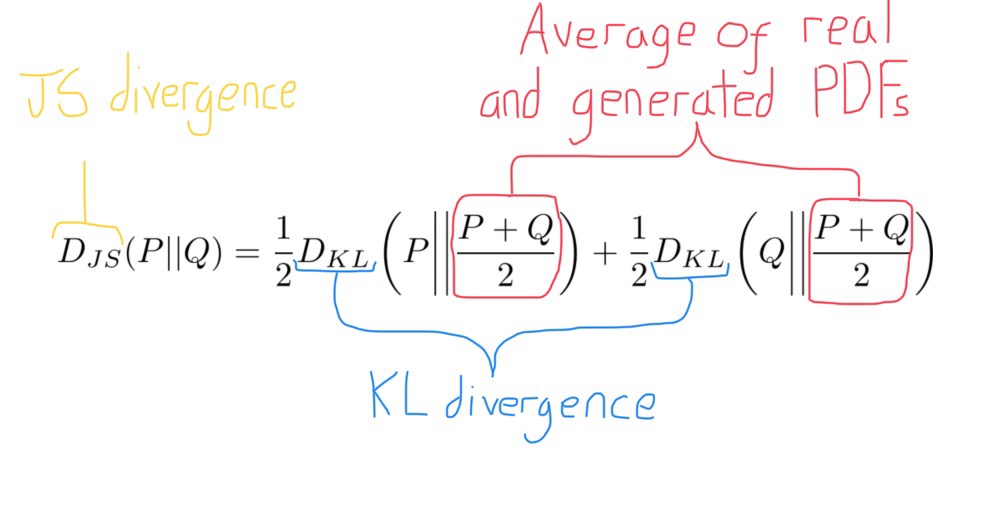
Jensen-Shannon divergence aims to address this asymmetry. Like KL divergence, it is a measure of similarity between two PDFs. However, unlike the KL divergence, you get the same result by swapping $P(x)$ and $Q(x)$. The JS divergence is therefore symmetric. Most GANs (as of 2018) aim to minimise a loss function that is equivalent to the JS divergence.
Sadly, the JS divergence is not the final stop on our journey to find a suitable loss function for our GAN. The nature of how probability distributions like $P(x)$ and $Q(x)$ manifest in high dimensions means that there will be many scenarios during training where either $P(x)$ or $Q(x)$ is 0 (we will explore this is more detail later). In these cases, the JS divergence experiences a sharp change and becomes non-differentiable. What is really needed is a loss function that is symmetric and smooth for all possible $P(x)$ and $Q(x)$. The Wasserstein distance is such a loss function.
Wasserstein Distance
The Wasserstein distance is symmetric, but to understand its main advantage we have to take a closer look at how both the real and generated data are distrubted in a multidimensional space. (Apologies if the following gets quite abstract/dense…)
Consider the following analogy. The universe we live in is a rather big 3-dimensional space. Humans, however, are only found in a very small part of that space, i.e Earth. Not only that but we are only found on the surface of the Earth, which appears as 2-dimensional to us humans. So humans only inhabit a small 2-dimensional space inside a much larger 3-dimensional space. In more mathematical terms, you can say that humans live on a 2-manifold inside a 3-dimensional space.
Now, in a slight change of direction, think about a stack of 128x128 pictures of Academy Award nominee Stanley Tucci.
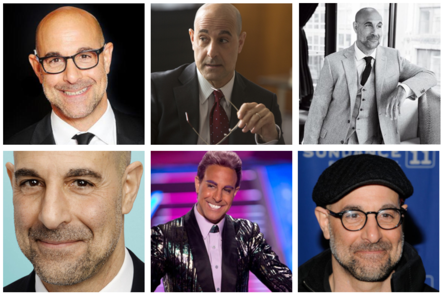
Each picture of Tucci has 128x128 = 16,384 individual pixels. (Let’s keep things simply and ignore RGB). By abstracting a bit, try and imagine a 16,384 dimensional space. Each point in the space corresponds to a different 128x128 picture. Moving along a single dimension in this space is equivalent to one pixel in our image changing value. Moreover, every possible 128x128 picture you can think of correspondse to a different point in this space, whether it be a cloud, a Piña Colada, or just some random noise.
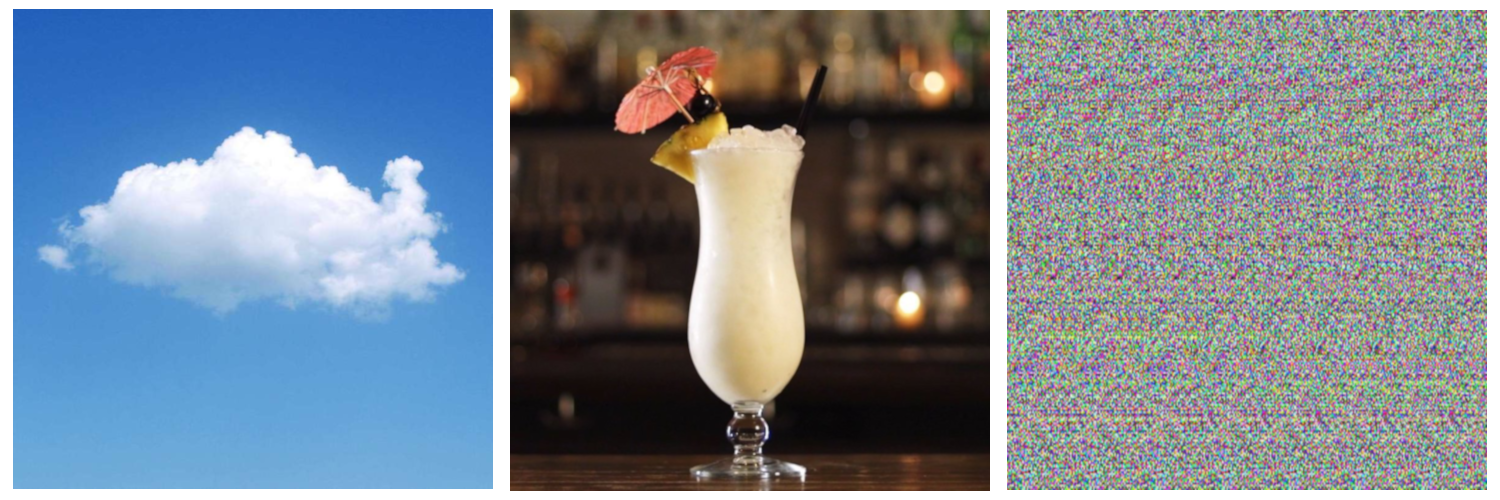
(Aside: It’s worth noting that nearly all points in our multi-dimensional space are going to correspond to an image that look something like the noise on the right. Points that have images with any structure or meaning will be very, very, very, very rare.)
In our 16,384 dimensional space, our real pictures of Tucci are going to only inhabit a very small space, most likely existsing on lower dimensional manifolds. This because there are far fewer 128x128 pictures of Tucci than there are possible 128x128 pictures.
If we are training a generator to produce pictures of Stanley then the generator’s output images are likely to exist on a separate set of manifolds in the 16,384 dimensional space. It is very, very unlikely that any of the real data’s manifolds and the generator’s manifolds are going to overlap in the multi-dimensional space. If this is the case then the probability distributions of the real and generated images are said to be disjoint.
Now we can finally get to why the Wasserstein distance is a better loss function for training GANs than the KL or JS divergences. In the likely situation where $P(x)$ and $Q(x)$ are disjoint, the KL and JS divergences often produce bad gradients, making training both the discriminator and generator very difficult. However, when we use the Wasserstein distance as a loss function, we get good gradients everywhere, even if the two probability distributions are disjoint.
Learning The Wasserstein Distance
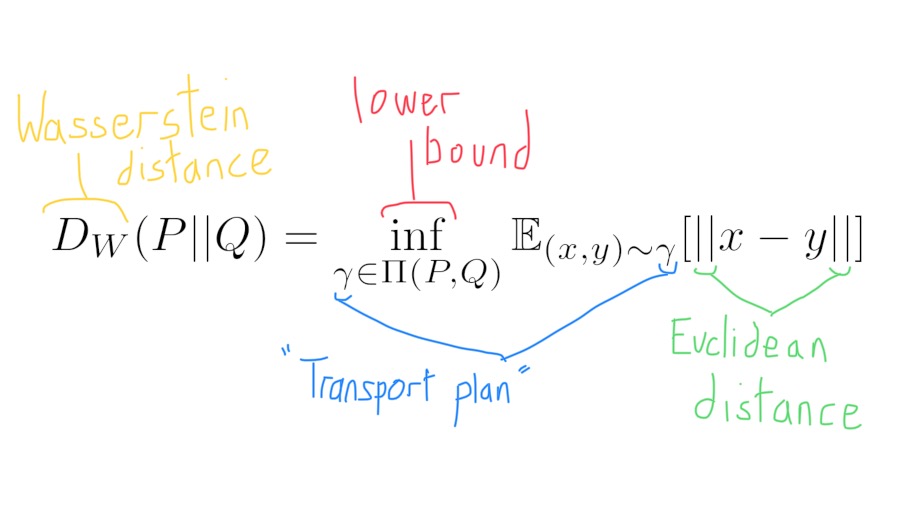
The above equation showing the Wasserstein distance is quite complicated. Annoyingly, it can’t be hand-written into your code like a more simple loss function like MSE. If coding the loss function isn’t possible then how can we possibly use it? This being machine learning, the answer should be obvious. We will use a neural network to learn the Wasserstein distance for itself!
This learning is possible using the Kantorovich-Rubinstein duality, which is a result that expresses the Wasserstein distance in another form:
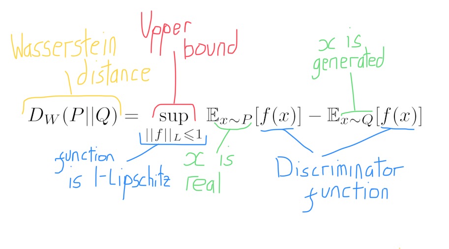
Take $f(x)$ to be the discriminator function (the discriminator takes in input $x$ and has an output $f(x)$). Consider the difference between what the discriminator outputs when it sees some real data and what it outputs when it sees some fake data. The Kantorovich-Rubenstein duality tells us that the upperbound of this difference is equal to the Wasserstein distance. This is a fairly remarkable result. However, it comes with a catch.
Lipschitz Functions
The catch is that the function our discriminator learns must belong to a specific family of functions, known as 1-Lipschitz functions. Although it sounds complicated, Lipschitz functions can be understood on a fairly intuitive level. If we have two points, $x_1$ and $x_2$, we can run them both through a function to get two new points, $y_1$ and $y_2$. If, for any $x_1$ and $x_2$ we select, the distance between $y_1$ and $y_2$ is less than or equal to the distance between $x_1$ and $x_2$ then our function is 1-Lipschitz.
The last piece in the jigsaw is making sure the function the discriminator learns is 1-Lipschitz. This is still an ongoing area of research. So far the different approaches taken have been fairly hacky. They include:
- Clipping the weights of all the weight matrices inside the discriminator so they stay within a fixed value. This is what was done in the original WGAN paper.
- Adding an extra term to our learnt Wasserstein distance loss function. This term penalises the discriminator if the norm of the gradients differ from 1. The resulting architecture is called WGAN-GP, the GP standing for Gradient-Penalty.
- Spectral normalisation. This idea is more theoretically sound than the methods above. Each weight matrix of the discriminator is normalised in proportion to its largest eigenvalue. Doing so limits the ‘stretchiness’ of each matrix and ensures they are 1-Lipschitz.